

How To Create A Dynamic Chart In Excel Using Vba
Bottom line: Learn how to automatically create more descriptive and dynamic chart titles that display the filter criteria with VBA macros.
Skill level: Intermediate
Video Tutorial
Pivot Chart Titles Default to Total
A chart's title should describe the data that is presented in the chart.
When inserting a new pivot chart, the chart's title usually defaults to the words "Total" or "Chart Title". This means we must always take extra steps to modify the chart title to make it more descriptive.
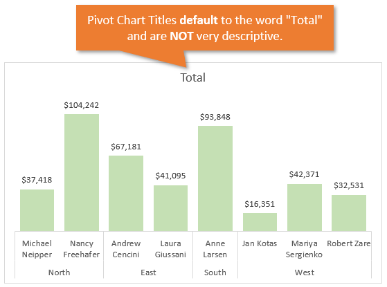
So, I wrote a few macros to automate this process, and also create dynamic titles that list the filter criteria.
Note: The macros just do the setup work, and are NOT actually needed for the interactive subtitles. More on that below.
If you're new to creating pivot tables and pivot charts, then checkout my free 3-part video series on pivot tables and dashboards.
The Automatic Chart Title Macros
The following macros create descriptive chart titles and dynamic subtitles for our Pivot Charts. The macros use the names (captions) of the fields used in the pivot chart to create the titles and subtitles.
Download the Excel File
You can download the Excel file that contains the macros below. The macros can be added to your Personal Macro Workbook.
![]() Dynamic PivotChart Title Macro.xlsm (266.0 KB)
Dynamic PivotChart Title Macro.xlsm (266.0 KB)
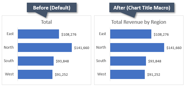
Macro #1: Auto Title PivotChart
The first macro creates a simple chart title based on the fields in the Values, Rows, and Columns areas of the pivot chart (pivot table).
The macro loops through each PivotField in the Values (DataFields), Rows (RowFields), and Columns (ColumnFields) of the PivotChart. It creates a string of text that joins together each field name (caption).
Note: The macro uses the Caption property of the pivot field, which is the field name that is displayed in the pivot table and chart. The Caption can be different from the Name property. The Name is the source (column) name from the source data.
The text uses separators between the values and rows/columns fields, which can be changed in the code. Here is an example of the structure of the title.
[Values Field Caption] by [Rows Field Caption] by [Columns Field Caption]
Here is an example of an actual title
Total Revenue by Salesperson by Quarter
The macro will include multiple fields in any of the areas, and list them in order of the field position. Here is an example.

[Values Field Caption] by [1st Rows Field Caption] by [2nd Rows Field Caption] by [Columns Field Caption]
If an area has multiple fields in the Values area, then the ampersand & is used to separate the field names.
Again, this is a simple macro that just saves time from having to type the chart title manually.
If you accidentally toggle the Chart Title checkbox on & off, then the chart title is reset to "Total". You typically have to re-type the title, but this macro will save time with that too.

Macro #2: Dynamic Pivot Chart Titles Textbox
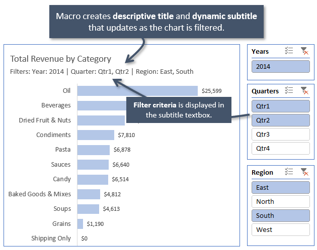
The second macro creates a dynamic subtitle to include the fields in the Filters area, and their filter criteria. This macro will save you a lot of time with manual setup work.
How the Macro Works
This macro is a bit more advanced. Here is a screencast of the macro in action.
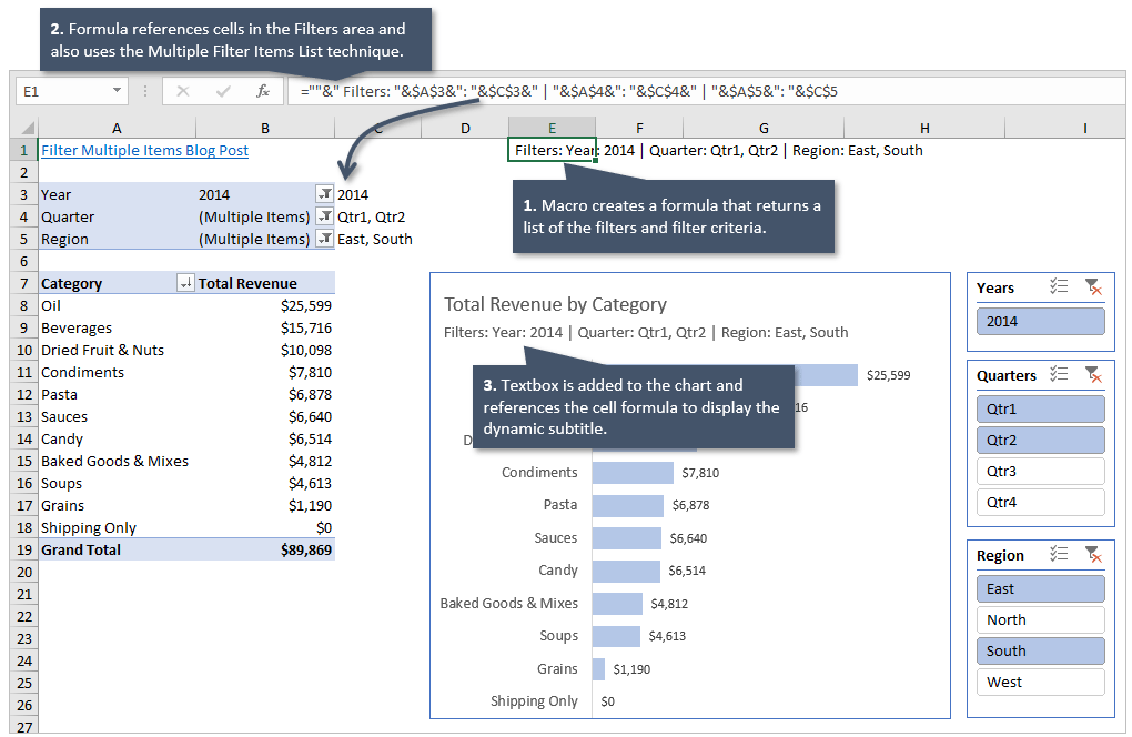
It first loops through the fields in the Filters Area of the pivot chart's pivot table and creates cell formula. The macro actually creates a string of text that references the cells in the Filters Area LabelRange (the cells in the pivot table that contain the filter fields and filter values (criteria).
The macro then displays an InputBox and prompts the user to select a blank cell for the formula. The formula is input in the sheet.
When the formula evaluates it will display a string of text that contains the filter fields and their criteria. Here is an example.
Filters: Year: 2014 | Quarter: Qtr1, Qtr2 | Region: East
A Textbox (shape) is added to the pivot chart for the subtitle. The textbox is linked to the cell that contains the formula. This is considered a dynamic title because the text in the textbox will change as the result of the formula changes.
Display Multiple Filter Items
In this example I'm also using another technique to display multiple filter items in a comma separated list. Checkout this post3 Ways to Display (Multiple Items) Filter Criteria in a Pivot Table to learn more.
When filters are applied to the pivot table/chart, the formula displays the filter criteria and so does the textbox.
Finally, the macro formats the textbox to match the text color of the chart's title. It also resizes the Plot Area of the chart to prevent the textbox from overlapping it.
The macro does a lot of work to create the chart's dynamic subtitle. The good news is that you don't have to do any of this manual setup work. Just run the macro!
It's important to note that the macro only does the setup work. Once the setup is complete the macro is no longer needed. The formula in the cell updates when the filters are applied, and the linked textbox in the chart just displays the cell's contents. This means that you do NOT need to store macros in the files that you run this macro on. This is nice if you are sending the files to other users and you don't want the file to contain macros.
Macro #3: Dynamic PivotChart Titles
The third macro just calls macro #1 and #2. You can use the macros independently if you only want to create a title or subtitle. Or, you can run them together to create both titles at the same time.
Add Macro Buttons to a Custom Ribbon
In the video above I run the macros from a custom "My Macros" ribbon. I created macro buttons that call the macros.
The macros are stored in my Personal Macro Workbook. This means I can run the macros on any pivot chart in any workbook I have open.
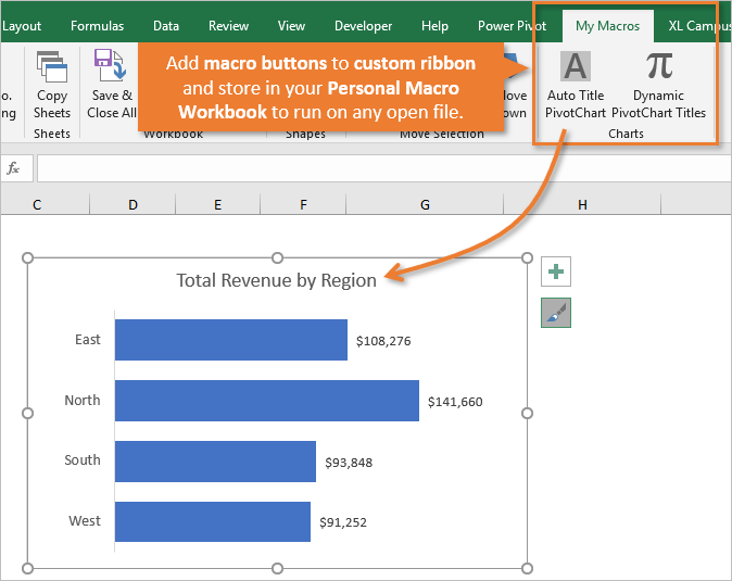
Once this is setup, you just have to select the chart, then press one of the macro buttons in the custom ribbon.
Checkout my 4-part video series on the Personal Macro Workbook to learn how to set it up and create the custom ribbons and buttons.
How Will You Use These Macros?
You can modify the macros to include additional formatting, title placement, etc. Checkout my Chart Alignment Add-in for more details on how to quickly move & align the chart elements.
Please leave a comment below with any questions or suggestions on how you would modify these macros. Thank you! 😊
How To Create A Dynamic Chart In Excel Using Vba
Source: https://www.excelcampus.com/vba/pivot-chart-title-macro/
Posted by: howlandthiled.blogspot.com
0 Response to "How To Create A Dynamic Chart In Excel Using Vba"
Post a Comment